When to Use
The Latin Square Design (LSD) extends the RCBD by controlling for two sources of variability simultaneously. Use it when:
- You have one treatment factor of interest.
- There are two blocking factors (e.g., rows and columns in a field, days and operators in a lab).
- The number of treatments equals the number of levels in each blocking factor (producing a square layout).
The Design
Each treatment appears exactly once in every row and every column. The model is:
where is the row effect, is the column effect, and is the treatment effect.
Data
We use a 4x4 Latin square dataset with four treatments, four rows, and four columns.
library(agrideshr)
data(lsd_data)
str(lsd_data)
#> Classes 'tbl_df', 'tbl' and 'data.frame': 16 obs. of 4 variables:
#> $ Row : Factor w/ 4 levels "1","2","3","4": 1 2 3 4 1 2 3 4 1 2 ...
#> $ Column : Factor w/ 4 levels "1","2","3","4": 1 4 3 2 2 1 4 3 3 2 ...
#> $ Treatment: Factor w/ 4 levels "1","2","3","4": 1 1 1 1 2 2 2 2 3 3 ...
#> $ Yield : num 8.7 7.3 5.1 8.7 9.2 7.5 6.7 4 11.6 12.7 ...
lsd_data
#> Row Column Treatment Yield
#> 1 1 1 1 8.7
#> 2 2 4 1 7.3
#> 3 3 3 1 5.1
#> 4 4 2 1 8.7
#> 5 1 2 2 9.2
#> 6 2 1 2 7.5
#> 7 3 4 2 6.7
#> 8 4 3 2 4.0
#> 9 1 3 3 11.6
#> 10 2 2 3 12.7
#> 11 3 1 3 14.0
#> 12 4 4 3 12.9
#> 13 1 4 4 9.1
#> 14 2 3 4 4.6
#> 15 3 2 4 9.2
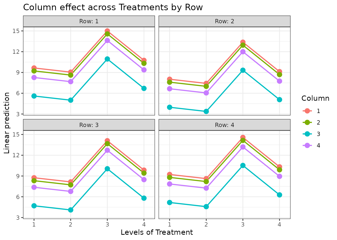
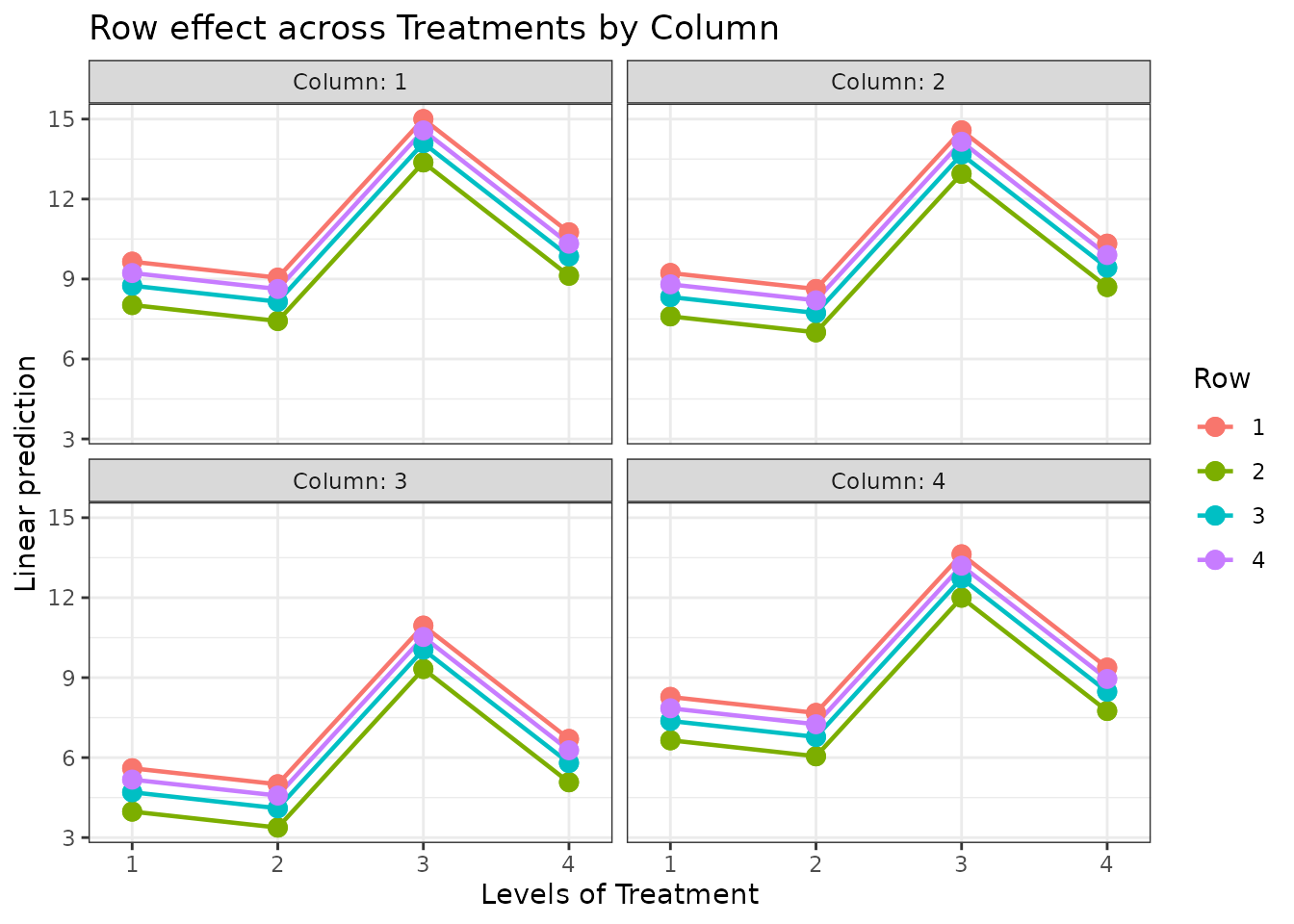
#> 16 4 1 4 11.3Exploratory Visualization
library(ggplot2)

ggplot(lsd_data, aes(x = Treatment, y = Yield, colour = Row, shape = Column)) +
  geom_point(size = 3) +
  ylim(0, NA) +
  theme_bw() +
  labs(title = "Yield by Treatment (Row and Column indicated)")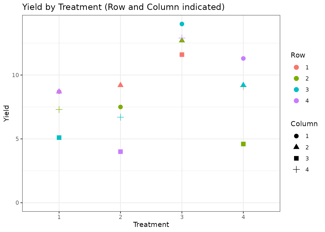
Model Fitting
Both row and column effects are included in the model:
mod <- aov(Yield ~ Row + Column + Treatment, data = lsd_data)
summary(mod)
#>             Df Sum Sq Mean Sq F value   Pr(>F)
#> Row          3   5.82   1.941   2.872 0.125712
#> Column       3  39.67  13.224  19.567 0.001683 **
#> Treatment    3  86.55  28.849  42.687 0.000193 ***
#> Residuals    6   4.06   0.676
#> ---
#> Signif. codes:  0 '***' 0.001 '**' 0.01 '*' 0.05 '.' 0.1 ' ' 1
The F-test for Treatment assesses treatment differences
after removing row and column variability.
Post-hoc Comparisons
We compare treatments only (rows and columns are nuisance factors):
TukeyHSD(mod, which = "Treatment")
#>   Tukey multiple comparisons of means
#>     95% family-wise confidence level
#>
#> Fit: aov(formula = Yield ~ Row + Column + Treatment, data = lsd_data)
#>
#> $Treatment
#>      diff        lwr       upr     p adj
#> 2-1 -0.60 -2.6123136  1.412314 0.7386088
#> 3-1  5.35  3.3376864  7.362314 0.0003869
#> 4-1  1.10 -0.9123136  3.112314 0.3224865
#> 3-2  5.95  3.9376864  7.962314 0.0002124
#> 4-2  1.70 -0.3123136  3.712314 0.0941779
#> 4-3 -4.25 -6.2623136 -2.237686 0.0013761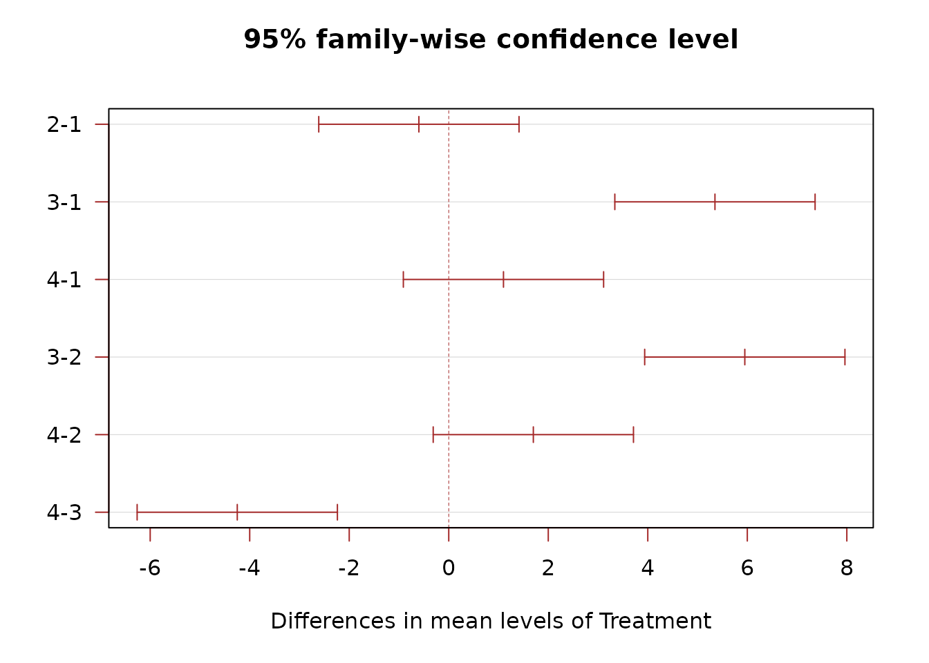
Estimated Marginal Means
library(emmeans)

emm <- emmeans(mod, specs = "Treatment")
emm
#>  Treatment emmean    SE df lower.CL upper.CL
#>  1           7.45 0.411  6     6.44     8.46
#>  2           6.85 0.411  6     5.84     7.86
#>  3          12.80 0.411  6    11.79    13.81
#>  4           8.55 0.411  6     7.54     9.56
#>
#> Results are averaged over the levels of: Row, Column
#> Confidence level used: 0.95
pairs(emm)
#>  contrast                estimate    SE df t.ratio p.value
#>  Treatment1 - Treatment2     0.60 0.581  6   1.032  0.7386
#>  Treatment1 - Treatment3    -5.35 0.581  6  -9.203  0.0004
#>  Treatment1 - Treatment4    -1.10 0.581  6  -1.892  0.3225
#>  Treatment2 - Treatment3    -5.95 0.581  6 -10.236  0.0002
#>  Treatment2 - Treatment4    -1.70 0.581  6  -2.924  0.0942
#>  Treatment3 - Treatment4     4.25 0.581  6   7.311  0.0014
#>
#> Results are averaged over the levels of: Row, Column
#> P value adjustment: tukey method for comparing a family of 4 estimates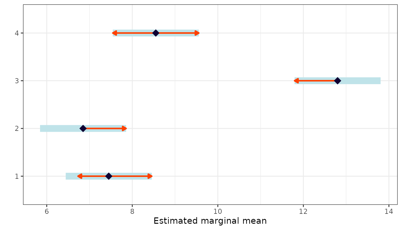
Conclusion
The Latin Square Design controls for two sources of heterogeneity simultaneously, making it highly efficient when the experimental layout naturally forms a grid. Limitations include:
- The number of treatments must equal the number of row and column levels.
- No interaction terms can be estimated (df are used for blocking).
When you need to study two treatment factors and their interaction, consider a Factorial Design.