Completely Randomized Design (CRD) • agrideshr

When to Use

The Completely Randomized Design (CRD) is the simplest experimental design. Use it when:

There is one treatment factor with two or more levels.
Experimental units are homogeneous (no known sources of variability to block).
Treatments are randomly assigned to units without restriction.

CRD is common in laboratory experiments and greenhouse trials where environmental conditions are uniform.

The Design

In a CRD, each treatment is assigned to experimental units purely at random. The statistical model is:

$Y_{ij} = \mu + \tau_i + \varepsilon_{ij}$

where $\mu$ is the overall mean, $\tau_i$ is the effect of treatment $i$ , and $\varepsilon_{ij} \sim N(0, \sigma^2)$ .

Data

We use a dataset comparing the yield of three squash varieties (Acorn, Butternut, Spaghetti) with three replicates each.

library(agrideshr)
data(crd_data)
str(crd_data)
#> Classes 'tbl_df', 'tbl' and 'data.frame':    9 obs. of  3 variables:
#>  $ Variety  : Factor w/ 3 levels "Acorn","Butternut",..: 3 3 3 2 2 2 1 1 1
#>  $ Replicate: Factor w/ 3 levels "rep1","rep2",..: 1 2 3 1 2 3 1 2 3
#>  $ Yield    : num  21.1 17.9 21.2 4.42 2.95 12.8 15.2 5.78 13.1
crd_data
#>      Variety Replicate Yield
#> 1 La Primera      rep1 21.10
#> 2 La Primera      rep2 17.90
#> 3 La Primera      rep3 21.20
#> 4  Butternut      rep1  4.42
#> 5  Butternut      rep2  2.95
#> 6  Butternut      rep3 12.80
#> 7      Acorn      rep1 15.20
#> 8      Acorn      rep2  5.78
#> 9      Acorn      rep3 13.10

Exploratory Visualization

library(ggplot2)

ggplot(crd_data, aes(x = Variety, y = Yield, fill = Variety)) +
  geom_boxplot(alpha = 0.7, outlier.shape = 16) +
  geom_jitter(width = 0.1, size = 2) +
  theme_bw() +
  labs(title = "Yield by Squash Variety", y = "Yield", x = "Variety") +
  theme(legend.position = "none")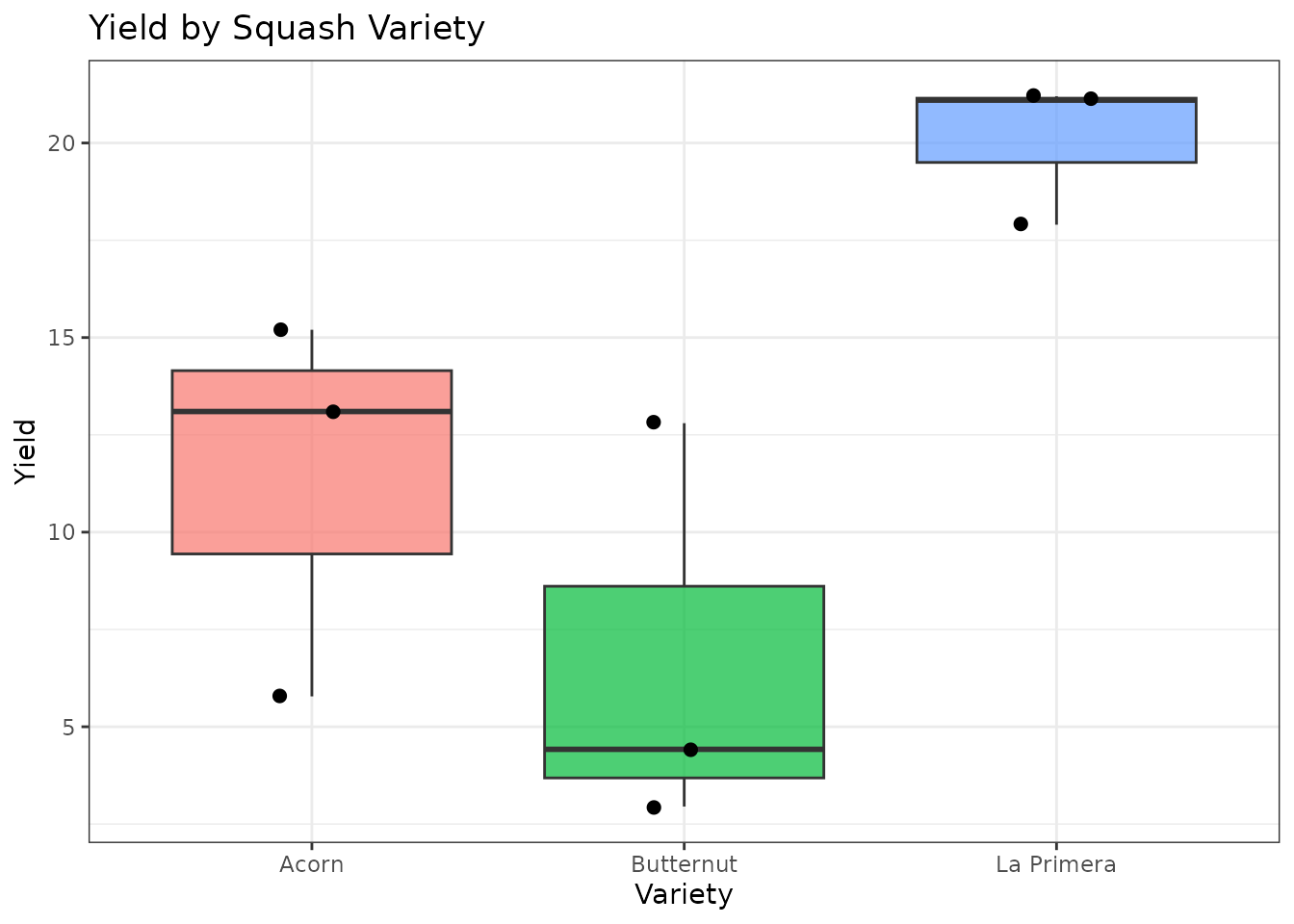

Descriptive statistics by variety:

library(dplyr)

crd_data %>%
  group_by(Variety) %>%
  summarise(
    N = n(),
    Mean = mean(Yield),
    SD = sd(Yield),
    .groups = "drop"
  )
#> # A tibble: 3 × 4
#>   Variety        N  Mean    SD
#>   <fct>      <int> <dbl> <dbl>
#> 1 Acorn          3 11.4   4.95
#> 2 Butternut      3  6.72  5.31
#> 3 La Primera     3 20.1   1.88

Model Fitting

We fit a one-way ANOVA using aov():

mod <- aov(Yield ~ Variety, data = crd_data)
summary(mod)
#>             Df Sum Sq Mean Sq F value Pr(>F)  
#> Variety      2  275.4  137.67   7.348 0.0244 *
#> Residuals    6  112.4   18.74                 
#> ---
#> Signif. codes:  0 '***' 0.001 '**' 0.01 '*' 0.05 '.' 0.1 ' ' 1

The F-test assesses whether at least one variety mean differs from the others.

Assumption Checking

ANOVA assumes that residuals are normally distributed and that variances are homogeneous across groups.

check_assumptions(mod, data = crd_data, group = "Variety")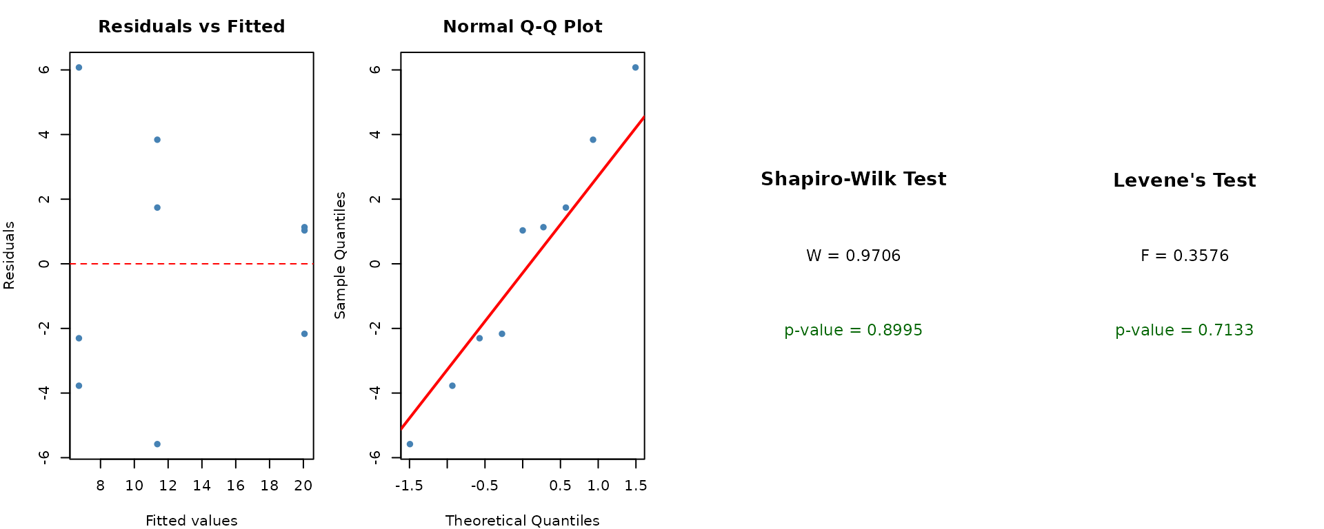

We can also check normality per group:

crd_data %>%
  group_by(Variety) %>%
  summarise(
    Shapiro_p = shapiro.test(Yield)$p.value,
    .groups = "drop"
  )
#> # A tibble: 3 × 2
#>   Variety    Shapiro_p
#>   <fct>          <dbl>
#> 1 Acorn         0.409 
#> 2 Butternut     0.265 
#> 3 La Primera    0.0509

Post-hoc Comparisons

If the F-test is significant, we compare varieties pairwise using Tukey’s HSD:

TukeyHSD(mod)
#>   Tukey multiple comparisons of means
#>     95% family-wise confidence level
#> 
#> Fit: aov(formula = Yield ~ Variety, data = crd_data)
#> 
#> $Variety
#>                           diff        lwr       upr     p adj
#> Butternut-Acorn      -4.636667 -15.481064  6.207731 0.4396163
#> La Primera-Acorn      8.706667  -2.137731 19.551064 0.1069483
#> La Primera-Butternut 13.343333   2.498936 24.187731 0.0215689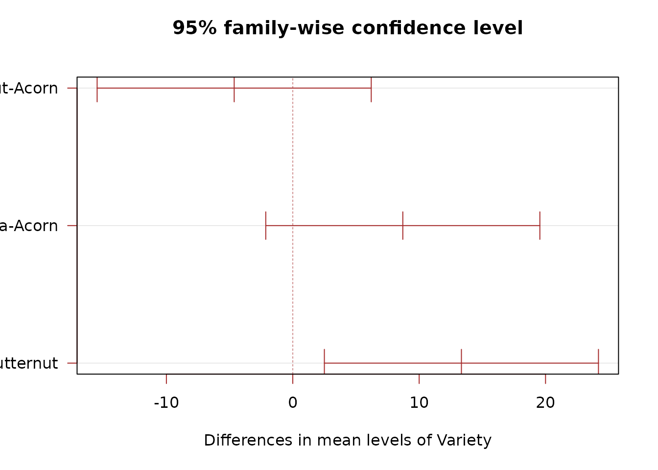

plot(TukeyHSD(mod), las = 1, col = "brown")

Estimated Marginal Means

The emmeans package provides estimated marginal means and pairwise contrasts:

library(emmeans)

emm <- emmeans(mod, specs = "Variety")
emm
#>  Variety    emmean  SE df lower.CL upper.CL
#>  Acorn       11.36 2.5  6    5.245     17.5
#>  Butternut    6.72 2.5  6    0.608     12.8
#>  La Primera  20.07 2.5  6   13.951     26.2
#> 
#> Confidence level used: 0.95

pairs(emm)
#>  contrast               estimate   SE df t.ratio p.value
#>  Acorn - Butternut          4.64 3.53  6   1.312  0.4396
#>  Acorn - La Primera        -8.71 3.53  6  -2.463  0.1069
#>  Butternut - La Primera   -13.34 3.53  6  -3.775  0.0216
#> 
#> P value adjustment: tukey method for comparing a family of 3 estimates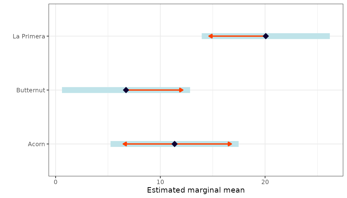

plot(emm, comparisons = TRUE) +
  theme_bw() +
  labs(y = "", x = "Estimated marginal mean")

Conclusion

The CRD analysis provides a straightforward way to compare treatment means when experimental units are homogeneous. The key outputs are:

F-test from the ANOVA table to detect overall differences.
Diagnostic plots to verify model assumptions.
Tukey HSD or emmeans contrasts for pairwise comparisons.

When experimental units are not homogeneous, consider using a Randomized Complete Block Design instead.