Randomized Complete Block Design (RCBD) • agrideshr

When to Use

The Randomized Complete Block Design (RCBD) is used when:

There is one treatment factor of interest.
There is a known source of variability (e.g., soil gradient, time, lab bench) that can be controlled by grouping units into blocks.
Each block contains all treatments exactly once.

RCBD reduces experimental error by accounting for block-to-block variability, making it more efficient than a CRD when conditions are not uniform.

The Design

The statistical model is:

$Y_{ij} = \mu + \beta_j + \tau_i + \varepsilon_{ij}$

where $\beta_j$ is the effect of block $j$ and $\tau_i$ is the treatment effect. Block effects are included to absorb known variability, but we are primarily interested in testing treatment differences.

Data

We use a dataset with six fertilizer levels (X25 through X150) applied across four blocks.

library(agrideshr)
data(rcbd_data)
str(rcbd_data)
#> Classes 'tbl_df', 'tbl' and 'data.frame':    24 obs. of  3 variables:
#>  $ Block    : Factor w/ 4 levels "1","2","3","4": 1 1 1 1 1 1 2 2 2 2 ...
#>  $ Treatment: Factor w/ 6 levels "X25","X50","X75",..: 1 2 3 4 5 6 1 2 3 4 ...
#>  $ Yield    : num  5.1 5.3 5.3 5.2 4.8 5.3 5.4 6 5.7 4.8 ...
head(rcbd_data, 12)
#>    Block Treatment Yield
#> 1      1       X25   5.1
#> 2      1       X50   5.3
#> 3      1       X75   5.3
#> 4      1      X100   5.2
#> 5      1      X125   4.8
#> 6      1      X150   5.3
#> 7      2       X25   5.4
#> 8      2       X50   6.0
#> 9      2       X75   5.7
#> 10     2      X100   4.8
#> 11     2      X125   4.8
#> 12     2      X150   4.5

Exploratory Visualization

library(ggplot2)

ggplot(rcbd_data, aes(x = Treatment, y = Yield, fill = Treatment)) +
  geom_boxplot(alpha = 0.7) +
  geom_jitter(width = 0.1, size = 2) +
  theme_bw() +
  labs(title = "Yield by Fertilizer Level", y = "Yield") +
  theme(legend.position = "none")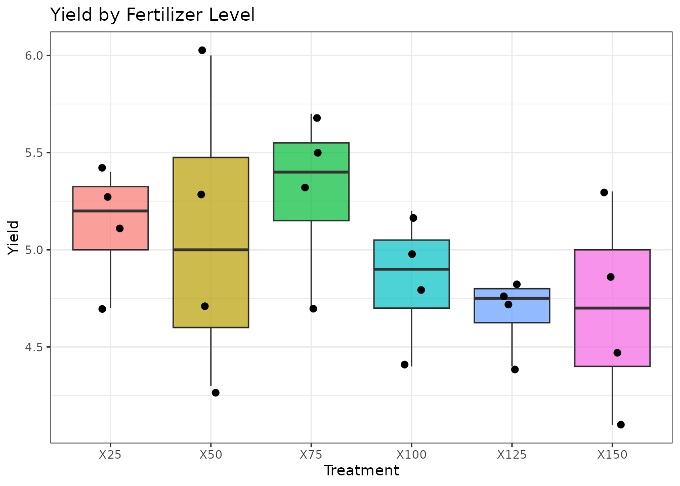

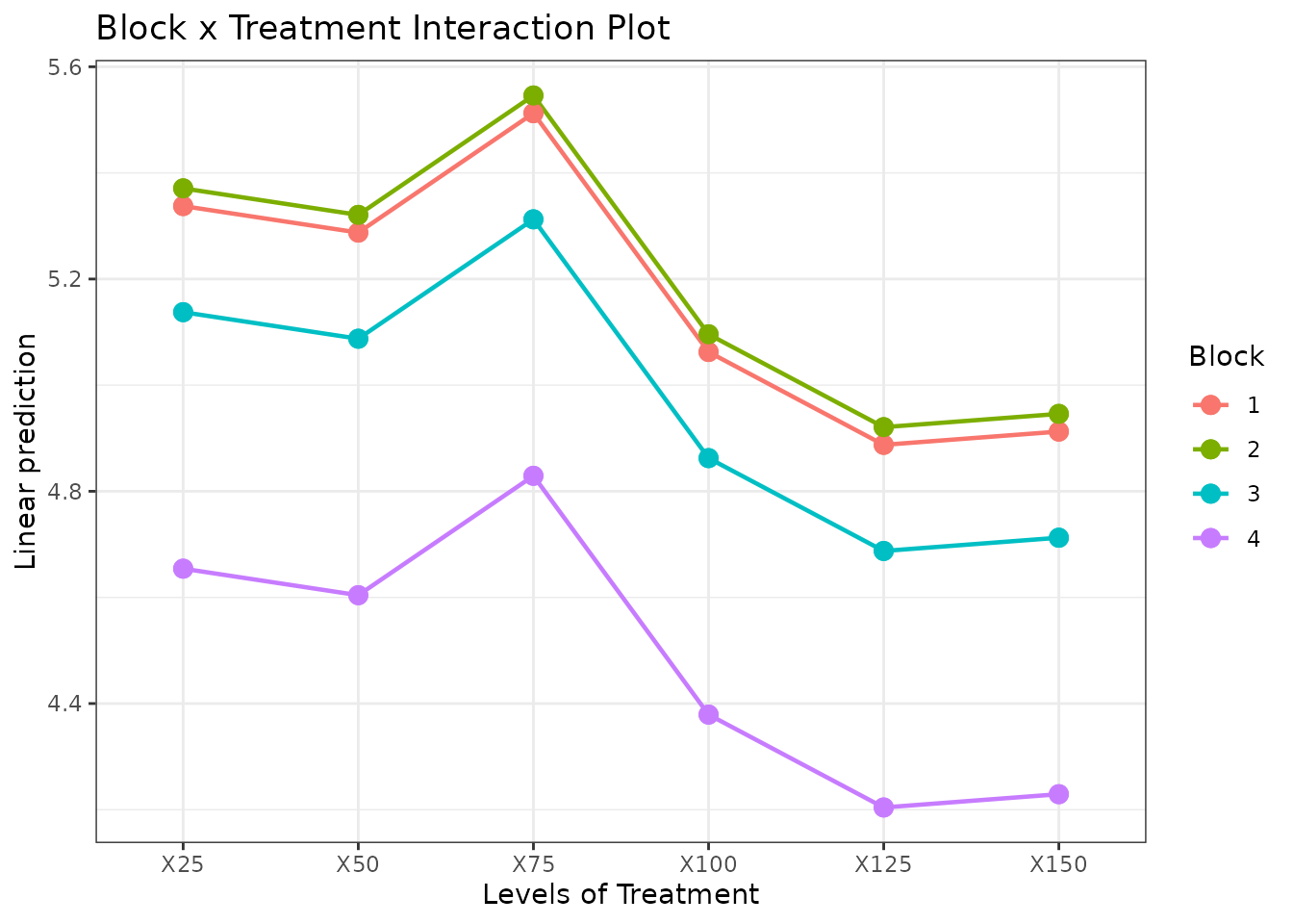
Treatment response by block:

ggplot(rcbd_data, aes(x = Treatment, y = Yield, colour = Block, group = Block)) +
  geom_point(size = 2) +
  stat_summary(fun = mean, geom = "line") +
  theme_bw() +
  labs(title = "Treatment Response by Block")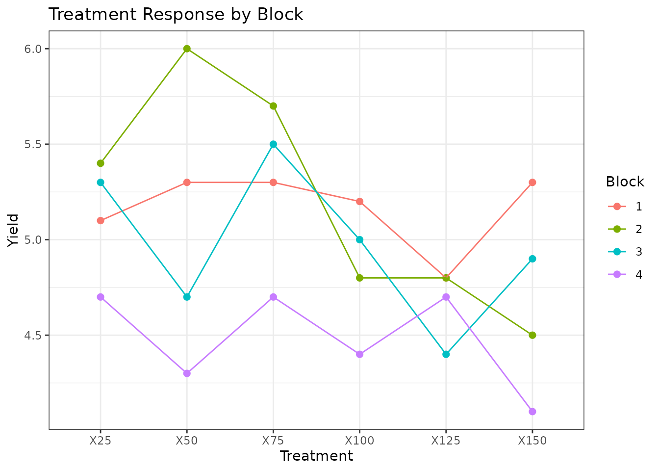

Model Fitting

In RCBD, the block is included as a factor in the model but is not the focus of inference:

mod <- aov(Yield ~ Block + Treatment, data = rcbd_data)
summary(mod)
#>             Df Sum Sq Mean Sq F value  Pr(>F)   
#> Block        3  1.965  0.6549   5.494 0.00949 **
#> Treatment    5  1.267  0.2534   2.126 0.11837   
#> Residuals   15  1.788  0.1192                   
#> ---
#> Signif. codes:  0 '***' 0.001 '**' 0.01 '*' 0.05 '.' 0.1 ' ' 1

The F-test for Treatment tells us whether fertilizer levels differ after accounting for block effects.

Assumption Checking

check_assumptions(mod, data = rcbd_data, group = "Treatment")

Post-hoc Comparisons

We compare treatments (not blocks) using Tukey’s HSD:

TukeyHSD(mod, which = "Treatment")
#>   Tukey multiple comparisons of means
#>     95% family-wise confidence level
#> 
#> Fit: aov(formula = Yield ~ Block + Treatment, data = rcbd_data)
#> 
#> $Treatment
#>             diff        lwr       upr     p adj
#> X50-X25   -0.050 -0.8431557 0.7431557 0.9999384
#> X75-X25    0.175 -0.6181557 0.9681557 0.9768219
#> X100-X25  -0.275 -1.0681557 0.5181557 0.8629753
#> X125-X25  -0.450 -1.2431557 0.3431557 0.4697141
#> X150-X25  -0.425 -1.2181557 0.3681557 0.5279646
#> X75-X50    0.225 -0.5681557 1.0181557 0.9347621
#> X100-X50  -0.225 -1.0181557 0.5681557 0.9347621
#> X125-X50  -0.400 -1.1931557 0.3931557 0.5879468
#> X150-X50  -0.375 -1.1681557 0.4181557 0.6483439
#> X100-X75  -0.450 -1.2431557 0.3431557 0.4697141
#> X125-X75  -0.625 -1.4181557 0.1681557 0.1678730
#> X150-X75  -0.600 -1.3931557 0.1931557 0.1980689
#> X125-X100 -0.175 -0.9681557 0.6181557 0.9768219
#> X150-X100 -0.150 -0.9431557 0.6431557 0.9882241
#> X150-X125  0.025 -0.7681557 0.8181557 0.9999980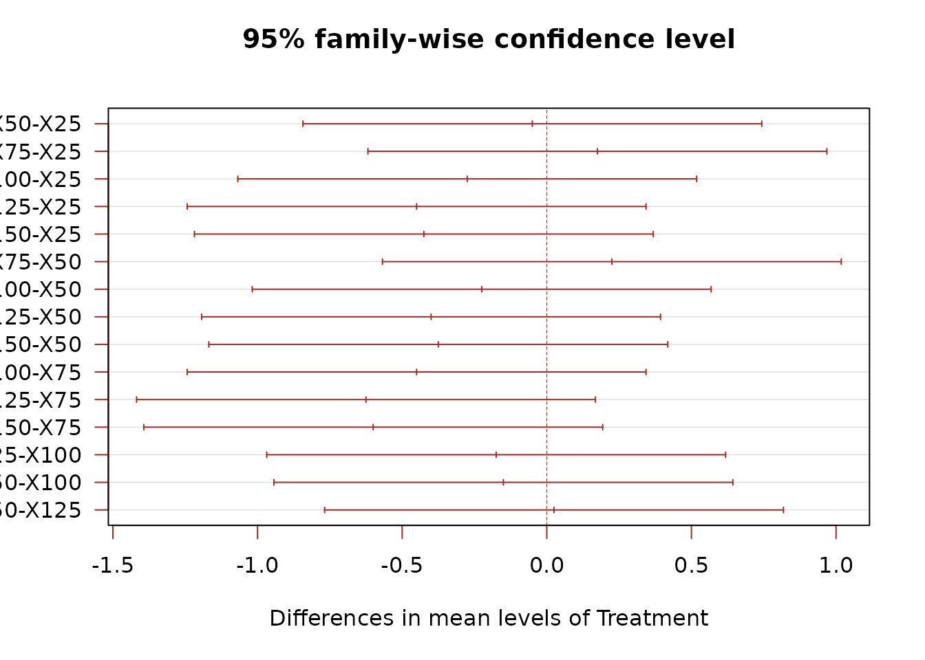

plot(TukeyHSD(mod, which = "Treatment"), las = 1, col = "brown")

Estimated Marginal Means

library(emmeans)

emm <- emmeans(mod, specs = "Treatment")
emm
#>  Treatment emmean    SE df lower.CL upper.CL
#>  X25         5.12 0.173 15     4.76     5.49
#>  X50         5.08 0.173 15     4.71     5.44
#>  X75         5.30 0.173 15     4.93     5.67
#>  X100        4.85 0.173 15     4.48     5.22
#>  X125        4.67 0.173 15     4.31     5.04
#>  X150        4.70 0.173 15     4.33     5.07
#> 
#> Results are averaged over the levels of: Block 
#> Confidence level used: 0.95

pairs(emm)
#>  contrast    estimate    SE df t.ratio p.value
#>  X25 - X50      0.050 0.244 15   0.205  0.9999
#>  X25 - X75     -0.175 0.244 15  -0.717  0.9768
#>  X25 - X100     0.275 0.244 15   1.126  0.8630
#>  X25 - X125     0.450 0.244 15   1.843  0.4697
#>  X25 - X150     0.425 0.244 15   1.741  0.5280
#>  X50 - X75     -0.225 0.244 15  -0.922  0.9348
#>  X50 - X100     0.225 0.244 15   0.922  0.9348
#>  X50 - X125     0.400 0.244 15   1.639  0.5879
#>  X50 - X150     0.375 0.244 15   1.536  0.6483
#>  X75 - X100     0.450 0.244 15   1.843  0.4697
#>  X75 - X125     0.625 0.244 15   2.560  0.1679
#>  X75 - X150     0.600 0.244 15   2.458  0.1981
#>  X100 - X125    0.175 0.244 15   0.717  0.9768
#>  X100 - X150    0.150 0.244 15   0.614  0.9882
#>  X125 - X150   -0.025 0.244 15  -0.102  1.0000
#> 
#> Results are averaged over the levels of: Block 
#> P value adjustment: tukey method for comparing a family of 6 estimates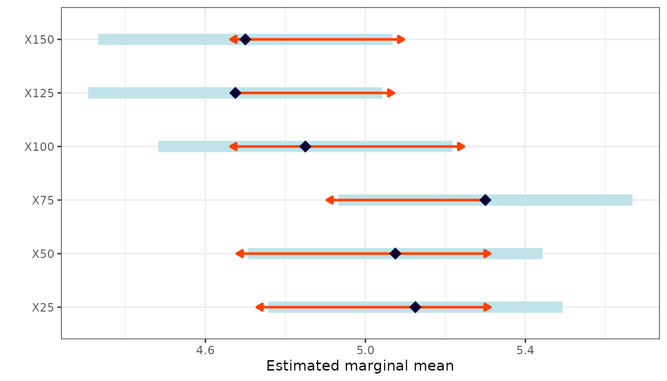

plot(emm, comparisons = TRUE) +
  theme_bw() +
  labs(y = "", x = "Estimated marginal mean")

Block-by-Treatment Interaction Plot

This plot helps visualise whether the treatment effect is consistent across blocks:

emmip(mod, Block ~ Treatment) +
  theme_bw() +
  labs(title = "Block x Treatment Interaction Plot")

Conclusion

The RCBD is the workhorse of agricultural experimentation. By blocking on a known source of variability, it provides a more precise estimate of treatment effects than a CRD. Key outputs:

ANOVA table with block and treatment effects separated.
Tukey HSD for pairwise treatment comparisons.
EMM interaction plots to check consistency across blocks.

When there are two sources of heterogeneity (e.g., rows and columns), consider a Latin Square Design.